Probabilistic Model Zoo
In this section, we present the code for implementing some models in InferPy.
Bayesian Linear Regression
Graphically, a (Bayesian) linear regression can be defined as follows,
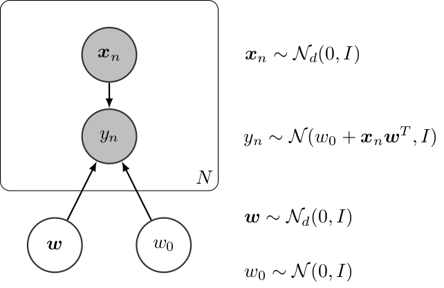
Bayesian Linear Regression
The InferPy code for this model is shown below,
import inferpy as inf
import tensorflow as tf
import numpy as np

@inf.probmodel
def linear_reg(d):
    w0 = inf.Normal(0, 1, name="w0")
    w = inf.Normal(np.zeros([d, 1]), 1, name="w")

    with inf.datamodel():
        x = inf.Normal(tf.ones(d), 2, name="x")
        y = inf.Normal(w0 + x @ w, 1.0, name="y")


@inf.probmodel
def qmodel(d):
    qw0_loc = inf.Parameter(0., name="qw0_loc")
    qw0_scale = tf.math.softplus(inf.Parameter(1., name="qw0_scale"))
    qw0 = inf.Normal(qw0_loc, qw0_scale, name="w0")

    qw_loc = inf.Parameter(np.zeros([d, 1]), name="qw_loc")
    qw_scale = tf.math.softplus(inf.Parameter(tf.ones([d, 1]), name="qw_scale"))
    qw = inf.Normal(qw_loc, qw_scale, name="w")


# create an instance of the model
m = linear_reg(d=2)
q = qmodel(2)
# create toy data
N = 1000
data = m.prior(["x", "y"], data={"w0": 0, "w": [[2], [1]]}, size_datamodel=N).sample()

x_train = data["x"]
y_train = data["y"]

# set and run the inference
VI = inf.inference.VI(qmodel(2), epochs=10000)
m.fit({"x": x_train, "y": y_train}, VI)


# extract the parameters of the posterior
m.posterior(["w", "w0"]).parameters()
Bayesian Logistic Regression
Graphically, a (Bayesian) logistic regression can be defined as follows,
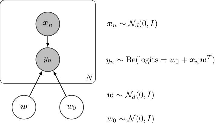
Bayesian Linear Regression
The InferPy code for this model is shown below,
import inferpy as inf
import numpy as np
import tensorflow as tf

d = 2
N = 10000


### Model definition ####

@inf.probmodel
def log_reg(d):
    w0 = inf.Normal(0., 1., name="w0")
    w = inf.Normal(np.zeros([d, 1]), np.ones([d, 1]), name="w")

    with inf.datamodel():
        x = inf.Normal(np.zeros(d), 2., name="x")  # the scale is broadcasted to shape [d] because of loc
        y = inf.Bernoulli(logits=w0 + x @ w, name="y")


@inf.probmodel
def qmodel(d):
    qw0_loc = inf.Parameter(0., name="qw0_loc")
    qw0_scale = tf.math.softplus(inf.Parameter(1., name="qw0_scale"))
    qw0 = inf.Normal(qw0_loc, qw0_scale, name="w0")

    qw_loc = inf.Parameter(tf.zeros([d, 1]), name="qw_loc")
    qw_scale = tf.math.softplus(inf.Parameter(tf.ones([d, 1]), name="qw_scale"))
    qw = inf.Normal(qw_loc, qw_scale, name="w")


##### Sample from prior model

# instance of the model
m = log_reg(d)

# create toy data
data = m.prior(["x", "y"], data={"w0": 0, "w": [[2], [1]]}).sample(N)
x_train = data["x"]
y_train = data["y"]


#### Inference

VI = inf.inference.VI(qmodel(d), epochs=10000)
m.fit({"x": x_train, "y": y_train}, VI)


#### Usage of the inferred model


# Print the parameters
w_post = m.posterior("w").parameters()["loc"]
w0_post = m.posterior("w0").parameters()["loc"]

print(w_post, w0_post)

# Sample from the posterior
post_sample = m.posterior_predictive(["x","y"], data={"w":w_post, "w":w0_post}).sample()
x_gen = post_sample["x"]
y_gen = post_sample["y"]

print(x_gen, y_gen)
Linear Factor Model (PCA)
A linear factor model allows to perform principal component analysis (PCA). Graphically, it can be defined as follows,

Linear Factor Model (PCA)
The InferPy code for this model is shown below,
# Generate toy data
x_train = np.concatenate([
    inf.Normal([0.0, 0.0], scale=1.).sample(int(N/2)),
    inf.Normal([10.0, 10.0], scale=1.).sample(int(N/2))
    ])
x_test = np.concatenate([
    inf.Normal([0.0, 0.0], scale=1.).sample(int(N/2)),
    inf.Normal([10.0, 10.0], scale=1.).sample(int(N/2))
    ])


# definition of a generic model
@inf.probmodel
def pca(k, d):
    beta = inf.Normal(loc=tf.zeros([k, d]),
                      scale=1, name="beta")               # shape = [k,d]

    with inf.datamodel():
        z = inf.Normal(tf.ones(k), 1, name="z")       # shape = [N,k]
        x = inf.Normal(z @ beta, 1, name="x")         # shape = [N,d]


@inf.probmodel
def qmodel(k, d):
    qbeta_loc = inf.Parameter(tf.zeros([k, d]), name="qbeta_loc")
    qbeta_scale = tf.math.softplus(inf.Parameter(tf.ones([k, d]),
                                                 name="qbeta_scale"))

    qbeta = inf.Normal(qbeta_loc, qbeta_scale, name="beta")

    with inf.datamodel():
        qz_loc = inf.Parameter(np.ones(k), name="qz_loc")
        qz_scale = tf.math.softplus(inf.Parameter(tf.ones(k),
                                                  name="qz_scale"))

        qz = inf.Normal(qz_loc, qz_scale, name="z")


# create an instance of the model and qmodel
m = pca(k=1, d=2)
q = qmodel(k=1, d=2)

# set the inference algorithm
VI = inf.inference.VI(q, epochs=2000)

# learn the parameters
m.fit({"x": x_train}, VI)

# extract the hidden encoding
Non-linear Factor Model (NLPCA)
Similarly to the previous model, the Non-linear PCA can be graphically defined as follows,

Non-linear PCA
Its code in InferPy is shown below,
import inferpy as inf
import tensorflow as tf

# definition of a generic model


# number of components
k = 1
# size of the hidden layer in the NN
d0 = 100
# dimensionality of the data
dx = 2
# number of observations (dataset size)
N = 1000


@inf.probmodel
def nlpca(k, d0, dx, decoder):

    with inf.datamodel():
        z = inf.Normal(tf.ones([k])*0.5, 1., name="z")    # shape = [N,k]
        output = decoder(z,d0,dx)
        x_loc = output[:,:dx]
        x_scale = tf.nn.softmax(output[:,dx:])
        x = inf.Normal(x_loc, x_scale, name="x")   # shape = [N,d]


def decoder(z,d0,dx):
    h0 = tf.layers.dense(z, d0, tf.nn.relu)
    return tf.layers.dense(h0, 2 * dx)


# Q-model  approximating P

@inf.probmodel
def qmodel(k):
    with inf.datamodel():
        qz_loc = inf.Parameter(tf.ones([k])*0.5, name="qz_loc")
        qz_scale = tf.math.softplus(inf.Parameter(tf.ones([k]),name="qz_scale"))

        qz = inf.Normal(qz_loc, qz_scale, name="z")


# create an instance of the model
m = nlpca(k,d0,dx, decoder)

# set the inference algorithm
VI = inf.inference.VI(qmodel(k), epochs=5000)

# learn the parameters
m.fit({"x": x_train}, VI)

# extract the hidden encoding
hidden_encoding = m.posterior("z").parameters()["loc"]

# project x_test into the reduced space (encode)
m.posterior("z", data={"x": x_test}).sample(5)

# sample from the posterior predictive (i.e., simulate values for x given the learnt hidden)
m.posterior_predictive("x").sample(5)

# decode values from the hidden representation
m.posterior_predictive("x", data={"z": [2]}).sample(5)
Variational auto-encoder (VAE)
Similarly to the PCA and NLPCA models, a variational auto-encoder allows to perform dimensionality reduction. However a VAE will contain a neural network in the P model (decoder) and another one in the Q (encoder). Its code in InferPy is shown below,
N = 1000

# Generate toy data
x_train = np.concatenate([
    inf.Normal([0.0, 0.0], scale=1.).sample(int(N/2)),
    inf.Normal([10.0, 10.0], scale=1.).sample(int(N/2))
    ])
x_test = np.concatenate([
    inf.Normal([0.0, 0.0], scale=1.).sample(int(N/2)),
    inf.Normal([10.0, 10.0], scale=1.).sample(int(N/2))
    ])


# number of components
k = 1
# size of the hidden layer in the NN
d0 = 100
# dimensionality of the data
dx = 2
# number of observations (dataset size)
N = 1000


@inf.probmodel
def vae(k, d0, dx, decoder):

    with inf.datamodel():
        z = inf.Normal(tf.ones(k) * 0.5, 1., name="z")    # shape = [N,k]
        output = decoder(z, d0, dx)
        x_loc = output[:, :dx]
        x_scale = tf.nn.softmax(output[:, dx:])
        x = inf.Normal(x_loc, x_scale, name="x")   # shape = [N,d]


def decoder(z, d0, dx):   # k -> d0 -> 2*dx
    h0 = tf.layers.dense(z, d0, tf.nn.relu)
    return tf.layers.dense(h0, 2 * dx)


# Q-model  approximating P
def encoder(x, d0, k):  # dx -> d0 -> 2*k
    h0 = tf.layers.dense(x, d0, tf.nn.relu)
    return tf.layers.dense(h0, 2 * k)


@inf.probmodel
def qmodel(k, d0, dx, encoder):

    with inf.datamodel():
        x = inf.Normal(tf.ones(dx), 1, name="x")

        output = encoder(x, d0, k)
        qz_loc = output[:, :k]
        qz_scale = tf.nn.softmax(output[:, k:])

        qz = inf.Normal(qz_loc, qz_scale, name="z")


# create an instance of the model
m = vae(k, d0, dx, decoder)
Note that in this example objects of class tf.layers are used, but
keras or tfp layers are compatible as well.