Bayesian Neural Networks

Neural networks are powerful approximators. However, standard approaches for learning this approximators does not take into account the inherent uncertainty we may have when fitting a model.

import logging, os
logging.disable(logging.WARNING)
os.environ["TF_CPP_MIN_LOG_LEVEL"] = "3"
import matplotlib.pyplot as plt
import numpy as np
import tensorflow as tf
import math
import inferpy as inf
import tensorflow_probability as tfp

Data

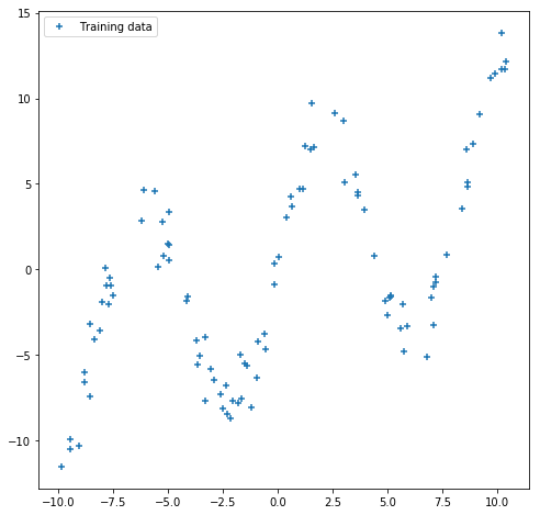
We use some fake data. As neural nets of even one hidden layer can be universal function approximators, we can see if we can train a simple neural network to fit a noisy sinusoidal data, like this:

NSAMPLE = 100
x_train = np.float32(np.random.uniform(-10.5, 10.5, (1, NSAMPLE))).T
r_train = np.float32(np.random.normal(size=(NSAMPLE,1),scale=1.0))
y_train = np.float32(np.sin(0.75*x_train)*7.0+x_train*0.5+r_train*1.0)

plt.figure(figsize=(8, 8))
plt.scatter(x_train, y_train, marker='+', label='Training data')
plt.legend();

Learning Standard Neural Networks

We employ a simple feedforward network with 20 hidden units to learn the model.

NHIDDEN = 20

nnetwork = tf.keras.Sequential([
    tf.keras.layers.Dense(NHIDDEN, activation=tf.nn.tanh),
    tf.keras.layers.Dense(1)
])

lossfunc = lambda y_out, y: tf.nn.l2_loss(y_out-y)

nnetwork.compile(tf.train.AdamOptimizer(0.01), lossfunc)
nnetwork.fit(x=x_train, y=y_train, epochs=1000)

Epoch 1/1000
100/100 [==============================] - 0s 2ms/sample - loss: 369.0472
Epoch 2/1000
100/100 [==============================] - 0s 110us/sample - loss: 333.4858
Epoch 3/1000
100/100 [==============================] - 0s 58us/sample - loss: 339.3102
    [...]
Epoch 997/1000
100/100 [==============================] - 0s 52us/sample - loss: 78.6340
Epoch 998/1000
100/100 [==============================] - 0s 50us/sample - loss: 78.3568
Epoch 999/1000
100/100 [==============================] - 0s 37us/sample - loss: 78.4461
Epoch 1000/1000
100/100 [==============================] - 0s 49us/sample - loss: 76.3849

<tensorflow.python.keras.callbacks.History at 0x139726668>

We see that the neural network can fit this sinusoidal data quite well, as expected.

sess = tf.keras.backend.get_session()
x_test = np.float32(np.arange(-10.5,10.5,0.1))
x_test = x_test.reshape(x_test.size,1)
y_test = sess.run(nnetwork(x_test))

plt.figure(figsize=(8, 8))
plt.plot(x_test, y_test, 'r-', label='Predictive mean');
plt.scatter(x_train, y_train, marker='+', label='Training data')
plt.xticks(np.arange(-10., 10.5, 4))
plt.title('Standard Neural Network')
plt.legend();

However, the model uncertainty is not appropriately captured. For example, when making predictions about a single point (e.g. around x=2.0), we can see we do not have into account the inherent noise there is in the prediction. In the next section, we will what happen when we introduce a Bayesian approach using InferPy.

Learning Bayesian Neural Networks

Bayesian modeling offers a systematic framework for reasoning about model uncertainty. Instead of just learning point estimates, we’re going to learn a distribution over variables that are consistent with the observed data.

In Bayesian learning, the weights of the network are random variables. The output of the nework is another random variable which is the one that implicitlyl defines the loss function. So, when making Bayesian learning we do not define loss functions, we do define random variables. For more information you can check this talk and this paper.

In Inferpy, defining a Bayesian neural network is quite straightforward. First we define the neural network using inf.layers.Sequential and layers of class tfp.layers.DenseFlipout. Second, the input x and output y are also defined as random variables. More precisely, the output y is defined as a Gaussian random varible. The mean of the Gaussian is the output of the neural network.

@inf.probmodel
def model(NHIDDEN):

    with inf.datamodel():
        x = inf.Normal(loc = tf.zeros([1]), scale = 1.0, name="x")

        nnetwork = inf.layers.Sequential([
            tfp.layers.DenseFlipout(NHIDDEN, activation=tf.nn.tanh),
            tfp.layers.DenseFlipout(1)
        ])

        y = inf.Normal(loc = nnetwork(x) , scale= 1., name="y")

To perform Bayesian learning, we resort to the scalable variational methods available in InferPy, which require the definition of a q model. For details, see the documentation about Inference in Inferpy. For a deeper theoretical despcription, read this paper. In this case, the q variables approximating the NN are defined in a transparent manner. For that reason we define an empty q model.

@inf.probmodel
def qmodel():
    pass

NHIDDEN=20

p = model(NHIDDEN)
q = qmodel()

VI = inf.inference.VI(q, optimizer = tf.train.AdamOptimizer(0.01), epochs=5000)

p.fit({"x": x_train, "y": y_train}, VI)

0 epochs    3477.63818359375....................
200 epochs  2621.487548828125....................
400 epochs  2294.40478515625....................
600 epochs  2003.2978515625....................
800 epochs  1932.5308837890625....................
1000 epochs         1912.515625....................
1200 epochs         1909.4072265625....................
1400 epochs         1908.7269287109375....................
1600 epochs         1908.28564453125....................
1800 epochs         1909.939697265625....................
2000 epochs         1907.779052734375....................
2200 epochs         1908.8096923828125....................
2400 epochs         1907.308349609375....................
2600 epochs         1907.8809814453125....................
2800 epochs         1906.529541015625....................
3000 epochs         1906.2943115234375....................
3200 epochs         1906.744140625....................
3400 epochs         1905.798828125....................
3600 epochs         1905.2296142578125....................
3800 epochs         1905.57275390625....................
4000 epochs         1905.6163330078125....................
4200 epochs         1904.5223388671875....................
4400 epochs         1904.778564453125....................
4600 epochs         1904.68408203125....................
4800 epochs         1903.94970703125....................

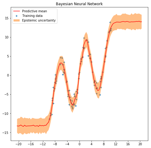
As can be seen in the next figure, the output of our model is not deterministic. So, we can capture the uncertainty in the data. See for example what happens now with the predictions at the point x=2.0. See also what happens with the uncertainty in out-of-range predictions.

x_test = np.linspace(-20.5, 20.5, NSAMPLE).reshape(-1, 1)

plt.figure(figsize=(8, 8))

y_pred_list = []
for i in range(100):
    y_test = p.posterior_predictive(["y"], data = {"x": x_test}).sample()
    y_pred_list.append(y_test)

y_preds = np.concatenate(y_pred_list, axis=1)

y_mean = np.mean(y_preds, axis=1)
y_sigma = np.std(y_preds, axis=1)

plt.plot(x_test, y_mean, 'r-', label='Predictive mean');
plt.scatter(x_train, y_train, marker='+', label='Training data')
plt.fill_between(x_test.ravel(),
                 y_mean + 2 * y_sigma,
                 y_mean - 2 * y_sigma,
                 alpha=0.5, label='Epistemic uncertainty')
plt.xticks(np.arange(-20., 20.5, 4))
plt.title('Bayesian Neural Network')
plt.legend();