Mixture Density Networks
Mixture density networks (MDN) (Bishop, 1994) are a class of models obtained by combining a conventional neural network with a mixture density model.
from __future__ import absolute_import
from __future__ import division
from __future__ import print_function

import inferpy as inf
import matplotlib.pyplot as plt
import numpy as np
import seaborn as sns
import tensorflow as tf
import tensorflow_probability as tfp

from scipy import stats
from sklearn.model_selection import train_test_split
def plot_normal_mix(pis, mus, sigmas, ax, label='', comp=True):
    """Plots the mixture of Normal models to axis=ax comp=True plots all
    components of mixture model
    """
    x = np.linspace(-10.5, 10.5, 250)
    final = np.zeros_like(x)
    for i, (weight_mix, mu_mix, sigma_mix) in enumerate(zip(pis, mus, sigmas)):
        temp = stats.norm.pdf(x, mu_mix, sigma_mix) * weight_mix
        final = final + temp
        if comp:
            ax.plot(x, temp, label='Normal ' + str(i))
    ax.plot(x, final, label='Mixture of Normals ' + label)
    ax.legend(fontsize=13)


def sample_from_mixture(x, pred_weights, pred_means, pred_std, amount):
    """Draws samples from mixture model.

    Returns 2 d array with input X and sample from prediction of mixture model.
    """
    samples = np.zeros((amount, 2))
    n_mix = len(pred_weights[0])
    to_choose_from = np.arange(n_mix)
    for j, (weights, means, std_devs) in enumerate(
                    zip(pred_weights, pred_means, pred_std)):
        index = np.random.choice(to_choose_from, p=weights)
        samples[j, 1] = np.random.normal(means[index], std_devs[index], size=1)
        samples[j, 0] = x[j]
        if j == amount - 1:
            break
    return samples
Data
We use the same toy data from David Ha’s blog post, where he explains MDNs. It is an inverse problem where for every input \(x_n\) there are multiple outputs \(y_n\).
def build_toy_dataset(N):
    y_data = np.random.uniform(-10.5, 10.5, N).astype(np.float32)
    r_data = np.random.normal(size=N).astype(np.float32)    # random noise
    x_data = np.sin(0.75 * y_data) * 7.0 + y_data * 0.5 + r_data * 1.0
    x_data = x_data.reshape((N, 1))
    return x_data, y_data

import random

tf.random.set_random_seed(42)
np.random.seed(42)
random.seed(42)

#inf.setseed(42)

N = 5000    # number of data points
D = 1    # number of features
K = 20    # number of mixture components

x_train, y_train = build_toy_dataset(N)


print("Size of features in training data: {}".format(x_train.shape))
print("Size of output in training data: {}".format(y_train.shape))
sns.regplot(x_train, y_train, fit_reg=False)
plt.show()
Size of features in training data: (5000, 1)
Size of output in training data: (5000,)

Fitting a Neural Network
We could try to fit a neural network over this data set. However, for each x value in this dataset there are multiple y values. So, it poses problems on the use of standard neural networks.
Let’s first define the neural network. We use tf.keras.layers to
construct neural networks. We specify a three-layer network with 15
hidden units for each hidden layer.
nnetwork = tf.keras.Sequential([
    tf.keras.layers.Dense(15, activation=tf.nn.relu),
    tf.keras.layers.Dense(15, activation=tf.nn.relu),
    tf.keras.layers.Dense(1, activation=None),
])
The following code fits the neural network to the data
lossfunc = lambda y_out, y: tf.nn.l2_loss(y_out-y)
nnetwork.compile(tf.train.AdamOptimizer(0.1), lossfunc)
nnetwork.fit(x=x_train, y=y_train, epochs=3000)
Epoch 1/3000
5000/5000 [==============================] - 0s 45us/sample - loss: 386.4314
Epoch 2/3000
5000/5000 [==============================] - 0s 24us/sample - loss: 360.6320
    [...]
Epoch 2997/3000
5000/5000 [==============================] - 0s 25us/sample - loss: 368.1469
Epoch 2998/3000
5000/5000 [==============================] - 0s 23us/sample - loss: 371.1811
Epoch 2999/3000
5000/5000 [==============================] - 0s 24us/sample - loss: 371.4650
Epoch 3000/3000
5000/5000 [==============================] - 0s 23us/sample - loss: 370.4930
<tensorflow.python.keras.callbacks.History at 0x135680198>
sess = tf.keras.backend.get_session()
x_test, _ = build_toy_dataset(200)
y_test = sess.run(nnetwork(x_test))

plt.figure(figsize=(8, 8))
plt.plot(x_train,y_train,'ro',x_test,y_test,'bo',alpha=0.3)
plt.show()
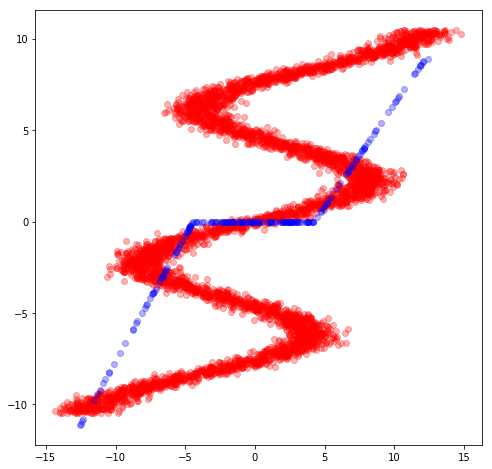
It can be seen, the neural network is not able to fit this data.
Mixture Density Network (MDN)
We use a MDN with a mixture of 20 normal distributions parameterized by a feedforward network. That is, the membership probabilities and per-component means and standard deviations are given by the output of a feedforward network.
We define our probabilistic model using InferPy constructs.
Specifically, we use the MixtureGaussian distribution, where the the
parameters of this network are provided by the feedforwrad network.
def neural_network(X):
    """loc, scale, logits = NN(x; theta)"""
    # 2 hidden layers with 15 hidden units
    net = tf.keras.layers.Dense(15, activation=tf.nn.relu)(X)
    net = tf.keras.layers.Dense(15, activation=tf.nn.relu)(net)
    locs = tf.keras.layers.Dense(K, activation=None)(net)
    scales = tf.keras.layers.Dense(K, activation=tf.exp)(net)
    logits = tf.keras.layers.Dense(K, activation=None)(net)
    return locs, scales, logits


@inf.probmodel
def mdn():
    with inf.datamodel():
        x = inf.Normal(loc = tf.ones([D]), scale = 1.0, name="x")
        locs, scales, logits = neural_network(x)
        y = inf.MixtureGaussian(locs, scales, logits=logits, name="y")

m = mdn()
Note that we use the MixtureGaussian random variable. It collapses
out the membership assignments for each data point and makes the model
differentiable with respect to all its parameters. It takes a list as
input—denoting the probability or logits for each cluster assignment—as
well as components, which are lists of loc and scale values.
For more background on MDNs, take a look at Christopher Bonnett’s blog post or at Bishop (1994).
Inference
Next we train the MDN model. For details, see the documentation about Inference in Inferpy
@inf.probmodel
def qmodel():
        return;

VI = inf.inference.VI(qmodel(), epochs=4000)
m.fit({"y": y_train, "x":x_train}, VI)
0 epochs    129578.296875....................
200 epochs  113866.8046875....................
400 epochs  110405.765625....................
600 epochs  108311.9296875....................
800 epochs  107741.84375....................
1000 epochs         106996.3359375....................
1200 epochs         106747.328125....................
1400 epochs         106299.640625....................
1600 epochs         106157.328125....................
1800 epochs         106087.8125....................
2000 epochs         106019.1875....................
2200 epochs         105955.0703125....................
2400 epochs         105751.9765625....................
2600 epochs         105717.4609375....................
2800 epochs         105693.375....................
3000 epochs         105676.3984375....................
3200 epochs         105664.40625....................
3400 epochs         105655.578125....................
3600 epochs         105648.265625....................
3800 epochs         105639.09375....................
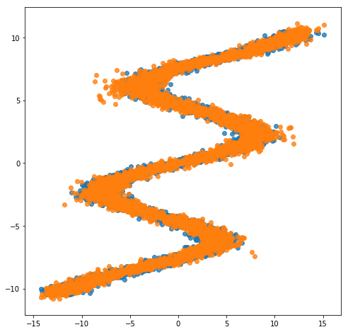
After training, we can now see how the same network embbeded in a mixture model is able to perfectly capture the training data.
X_test, y_test = build_toy_dataset(N)
y_pred = m.posterior_predictive(["y"], data = {"x": X_test}).sample()

plt.figure(figsize=(8, 8))
sns.regplot(X_test, y_test, fit_reg=False)
sns.regplot(X_test, y_pred, fit_reg=False)
plt.show()
Acknowledgments
This tutorial is inspired by David Ha’s blog post and Edward’s tutorial.